Theoretically, the order of the summation doesn’t matter. However, in computations it is better to sum over k before j, to avoid propagating large derivative matrices in the forward direction. This reverse flow for the derivative calculation, shown in Fig. 1 as the dashed arrows, is called the adjoint differentiation calculation.

Figure 1. A data-flow diagram describing a sequence of transforms of an input data vector x into a scalar output functional j. The data structures x, y and z may be large. Derivatives of j with respect to x are most efficiently evaluated by propagating derivatives of j with respect to the intermediate variables in the reverse (adjoint) direction (dashed lines).
In the modular approach implied by Fig. 1, each box represents a software module that performs a particular transformation of the input data to produce output data. In this approach adjoint differentiation can be achieved relatively easily. The only requirement is that each module not only be able to perform its forward transformation, but also be able to calculate the derivative of its outputs with respect to its inputs. The forward simulation process is achieved by linking together the necessary modules. The output of the simulation is the objective function to be minimised, for example, the measure of mismatch to some given measurements. The data-flow diagram (network or graph) that describes the forward calculation automatically provides the path for the reverse or adjoint calculation needed to accumulate the sensitivities of the objective function to any parameters in the simulation model. In this framework, the sensitivities of the output objective function with respect to all the simulation parameters can be automatically calculated in a time that is comparable to the forward simulation calculation.
3. BAYES INFERENCE ENGINE
The Bayes Inference Engine (BIE) provides a superb example of the modular approach to modelling and sensitivity analysis. The BIE is a computer application for analysing radiographs and making inferences about an object being radiographed [3]. The BIE is a graphical programming tool that automatically implements adjoint differentiation, which facilitates advanced model building and allows hundreds or thousands of parameters to be determined by matching a radiograph in a reasonable time.
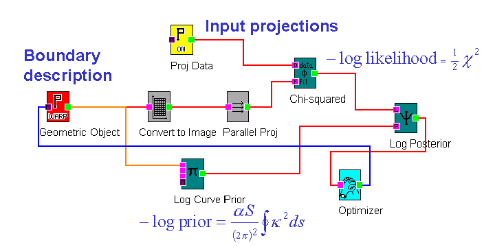
The BIE represents a computational approach to Bayesian inference, as opposed to the traditional analytical approach. The computational approach affords great flexibility in modelling, which facilitates the construction of complex models. The BIE easily deals with data that are nonlinearly dependent on the model parameters. Furthermore, the computational approach allows one to use nonGaussian probability distributions, such as likelihood functions based on Poisson distributions. Figure 2 shows the canvas of the BIE for a tomographic reconstruction problem in which three projections of a 2D object are used to determine the shape of the object. The reconstructed object is modelled as a uniform (known) density inside a flexible boundary, specified in terms of a 60-sided polygon. A smoothness prior is placed on the boundary. The BIE’s automatic adjoint differentiation permits the 120 variables to be determined in 20 optimiser iterations, or in a time corresponding to around 50 forward-model evaluations.
The BIE is designed and programmed within an object-oriented framework in which it id easy to make connections work in the reverse direction. An interesting aspect of the BIE is that there is no supervisory code. The modules act autonomously by responding to requests from other modules that are connected to their output for updated results. Each module asks its inputs for current information and then does its own calculation. It is the module at the end of the calculation, the optimiser in Fig. 2, that initiates the requests and finally gets the results of the calculation. The parameter modules (boxes labelled as P) terminate requests for forward calculations. This modular approach greatly simplifies adjoint calculations. The reverse flow of the derivatives proceeds in much the same manner. Figure 3 shows the result of a nonlinear optimisation.

Figure 2. A canvas from the BIE showing a data-flow diagram composed to simulate a radiographic measurement of an object that is defined in terms of a geometric description of its boundary. The minus-log-likelihood is added to a minus-log-prior to obtain a minus-log-posterior, which is to be minimised with respect to the geometry. Derivatives of the minus-log-posterior with respect to the geometric parameters are automatically calculated in the BIE in a computational time that is comparable to the forward simulation calculation.


Figure 3. An optimisation achieved with the BIE with the diagram shown in Fig. 2. Three noisy projections of the original object (left) are available, making this a very difficult reconstruction problem. The image on the right represents the shape that minimises the minus-log-posterior on the right in Fig. 2, obtained by varying the 120 parameters that describe its geometric boundary.
4. DISSCUSION
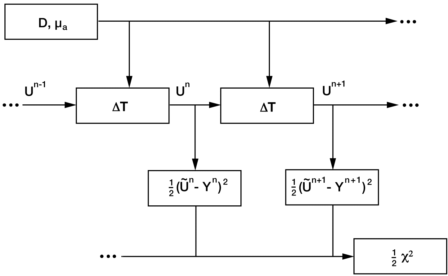
The modular approach to adjoint sensitivity calculation incorporated in the BIE can readily be applied to other simulation applications. References [4] and [5] demonstrate the use of adjoint differentiation to solve a complex inversion problem involving the diffusion of infrared light in tissue. Figure 4 shows the data-flow diagram, which could be used as a basis for creating the modular design described above.

Figure 4. A data-flow diagram for the simulation of a time-dependent diffusion process. The parameters in the upper-left hand box, the position-dependent diffusion constant and absorption coefficient, control the diffusion. The DT boxes provide the time-step calculation for the light-intensity field U, which is sampled to compare to time-dependent measurements. The output of the calculation is the scalar c2/2, which is to be minimised to obtain the best match to the measurements. The minimisation is efficiently accomplished through use of the gradients calculated by the adjoint method, which follows the direction of the dashed arrows.
Adjoint sensitivities are only not useful for optimisation, but also for drawing inferences about the uncertainties in model parameters. For example, the Hamiltonian method of Markov Chain Monte Carlo [6] uses the gradient of the minus-log-posterior function. MCMC is implemented in the BIE by replacing the optimiser by an MCMC module.
ACKNOWLEDGEMENTS
For many valuable interactions and collaborations, we would like to thank Rudy Henninger, Maria Rightley, Xavier Battle, Suhail Saquib, Andreas Hielscher, and Alex Klose. This work was supported by US-DOE under contract W-7405-ENG-36.
REFERENCES
- Hanson, KM, Cunningham (1998), Inversion based on computational simulations, Maximum Entropy and Bayesian Methods, pp. 121-135, Kluwer Academic, Dordrecht. (abstract: http://public.lanl.gov/kmh/publications/maxent97.abs.html)
- Giering, R (1997), Tangent-linear and Adjoint Model Compiler, Tech. Report TAMC 4.7, Max-Planck-Institut für Meterologie.
- Hanson, KM, Cunningham (1999), Operation of the Bayes Inference Engine, Maximum Entropy and Bayesian Methods, pp. 309-318, Kluwer Academic, Dordrecht. (abstract: http://public.lanl.gov/kmh/publications/maxent98.abs.html)
- Saquib, SS, Hanson, KM, Cunningham, GS (1997), Model-based image reconstruction from time-resolved diffusion data, Medical Imaging: Image Processing, Proc. SPIE 3338, pp. 369-380. (abstract: http://public.lanl.gov/kmh/publications/medim97b.abs.html)
- Hielscher, AH, Klose, AD, Hanson, KM (1999), Gradient-based iterative image reconstruction scheme for time-resolved optical tomography, IEEE Trans. Med. Imag. 18, pp. 262-271. (abstract: http://public.lanl.gov/kmh/publications/tmi99a.abs.html)
- Hanson, KM (2001), Markov Chain Monte Carlo posterior sampling with the Hamiltonian method, Proc. Sensitivity Analysis of Model Output, P. Prado, ed. (abstract: http://public.lanl.gov/kmh/publications/samo01a.abs.html)