Los Alamos National Laboratory, MS P940, Los Alamos, NM 87545 (USA)
Email: kmh@hansonhub.com, WWW: http://public.lanl.gov/kmh/

A major advantage of Bayesian data analysis is that provides a characterisation of the uncertainty in the model parameters estimated from a given set of measurements in the form of a posterior probability distribution [1]. When the analysis involves a complicated physical phenomenon, the posterior may not be available in analytic form, but only calculable by means of a simulation code. In such cases, the uncertainty in inferred model parameters requires characterisation of a calculated functional. An appealing way to explore the posterior, and hence characterise the uncertainty, is to employ the Markov Chain Monte Carlo technique. The goal of MCMC is to generate a sequence random of parameter x samples from a target pdf (probability density function), p(x). In Bayesian analysis, this sequence corresponds to a set of model realisations that follow the posterior distribution [2].

There are two basic MCMC techniques. In Gibbs sampling, typically one parameter is drawn from the conditional pdf at a time, holding all others fixed. In the Metropolis algorithm, all the parameters can be varied at once. The parameter vector is perturbed from the current sequence point by adding a trial step drawn randomly from a symmetric pdf. The trial position is either accepted or rejected on the basis of the probability at the trial position relative to the current one. The Metropolis algorithm is often employed because of its simplicity.

The aim of this work is to develop MCMC methods that are useful for large numbers of parameters, n, say hundreds or more. In this regime the Metropolis algorithm can be unsuitable, because its efficiency drops as 0.3/n [3]. The efficiency is defined as the reciprocal of the number of steps in the sequence needed to effectively provide a statistically independent sample from p.

An alternative MCMC technique is what I will call the Hamiltonian method. It is often referred to as the hybrid method because it alternates between Gibbs and Metropolis steps, but that name is not distinctive. For each parameter x_i, another parameter p_i is introduced, which represents the parameter's conjugate momentum variable [4]. A Hamiltonian is constructed as a potential term j = -log(p(x)), plus a kinetic energy term:
(1)
where m_i is a fictitious mass. The goal is to draw random samples from the new pdf that is proportional to exp(-H). Each iteration of the algorithm starts with a Gibbs sampling to pick a new momentum vector from the uncorrelated Gaussian in the momenta corresponding to the second term in H. Then a trajectory in (x,p) space is followed such that H is constant using the leapfrog technique, which consists of the following three substeps:
(2)
(3)
(4)
The parameter t represents an increment in time. After m leapfrog steps corresponding to a total trajectory time of T = mt, a Metropolis acceptance/rejection decision is made to guarantee that the sequence is in statistical equilibrium with the target pdf. Clearly large steps in the parameter space are possible with only a few evaluations of j and the gradient of j . Note that the gradient of j can often be done in a time comparable to the (forward) calculation of j by applying adjoint differentiation to the computer code used to calculate j [5]. In practice, the length of the Hamiltonian trajectories must be randomised to realise adequate sampling of p(x). Once an MCMC sequence has been generated, the properties of p(x) may be characterised by considering just the x samples. The momentum aspects of the extended pdf, exp(-H), are marginalised out because they are independent of the x dependence.

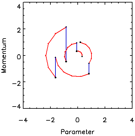
Figure 1 shows typical paths followed by the Hamiltonian MCMC algorithm for a one-dimensional target pdf, which is a Gaussian with unit standard deviation. The vertical jumps correspond to the Gibbs sampling of momentum from the Gaussian pdf, exp(-p²), for unity mass. The circular arcs correspond to the trajectories of constant H followed in five steps of the leapfrog method using t = 0.4, yielding a total trajectory length of T = 5t = 2.

Figure 1. Example of several trajectories in the momentum-parameter space for the Hamiltonian method for a 1D Gaussian distribution. For each trajectory, the momentum is drawn from the assumed Gaussian momentum distribution (vertical jumps), which is followed by several steps along a trajectory of constant Hamiltonian value (circular paths).

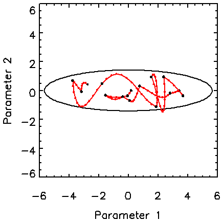
Figure 2 shows the behaviour of the Hamiltonian method for an asymmetric two-dimensional Gaussian distribution with a standard deviation of four in one direction and unity in the other. For this example, the maximum value for t is 0.4. The total length of each Hamiltonian trajectory is randomly chosen from a distribution that is uniform from 0 to T_max = 5 and t is adjusted for a minimum number of number of leapfrog steps. The important aspect of this example is that the full width of the target pdf is easily reached in relatively few (15) trajectories consisting of 91 leapfrog steps. This kind of distribution causes difficulty for the Metropolis algorithm with an isotropic trial distribution because it essentially follows a random walk.

Figure 2. Hamiltonian trajectories for a two-dimensional asymmetric uncorrelated Gaussian pdf, demonstrating the ability of the Hamiltonian trajectories to readily transverse the length of the target pdf.

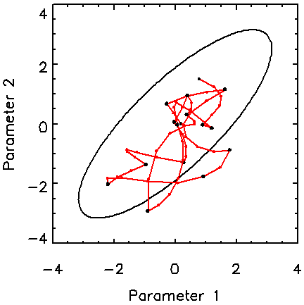
The motivation here is to handle pdfs of high dimensionality. Figure 3 shows how the Hamiltonian method copes with a 16D Gaussian distribution with a fair degree of correlation among the variables. The covariance matrix of the target pdf is a circulant matrix with rows whose elements are –0.2, 0.0, 0.4, 1.2, 2.5, 4.0, 5.0, 4.0, 2.5, 1.2, 0.4, 0.0, -0.2, with the maximum value on the diagonal [6]. The figure shows that the Hamiltonian method does a good job of sampling this pdf with only 15 trajectories, or 61 function and gradient evaluations. The maximum Hamiltonian length is 3 for this example.

Figure 3. Trajectories in a 2D subspace from a 16-dimensional correlated Gaussian pdf. The contour shown is at the two-standard-deviation level for the marginalised distribution.

The efficiency of Hamiltonian method is found to be optimised for t = 0.4 and T_max = 8. The MCMC algorithm is tested by running the algorithm 1000 times with 50 Hamiltonian trajectories in each run. The efficiency of the algorithm is calculated as the ratio of the mean square deviation from the mean of the parameter variance expected for ideal independent sampling method to that observed for the 1000 runs. The efficiency of the Hamiltonian method under these conditions is 45% per Hamiltonian trajectory or 2.1% per function evaluation. The latter number assumes that the computation time for gradient computation of j is the same as for j itself, which is often possible when the gradient is calculated using a code that represents the adjoint differentiation of the simulation code [5]. In the examples shown in Figs. 1 and 2, the Hamiltonian trajectories maintain constant H so that the Metropolis rejection rate is nearly zero. However, in this example, about 8% of the trajectories are rejected.

The previous problem involving a target distribution with modest correlations was treated in [6]. Using an isotropic trial distribution in the Metropolis algorithm, the efficiency was determined to be 0.11%. When the trial distribution is adaptively modified to have a covariance structure similar to that of the target pdf, the efficiency improved to 1.6%. This latter efficiency is close to the upper limit on efficiency of the simple Metropolis algorithm for a 16D isotropic pdf, 1.9%.

Comparison of these results with those for the Hamiltonian method indicates that the Hamiltonian method has the advantage of providing good efficiency without the need to supply an estimate of the covariance method. Furthermore, as the number of dimensions increases, the efficiency of the simple Metropolis algorithm will drop as 0.3/n. On the other hand, for pdfs in 64 dimensions with the same pdf, the efficiency of the Hamiltonian method is 1.9% per function evaluation and for 128 dimensions, it is 1.7%. Thus, the Hamiltonian MCMC method appears to be well suited for sampling pdfs of high dimension.

Almost the entire drop in efficiency comes from the Metropolis rejection of the Hamiltonian trajectories, which is the deterministic part of the algorithm. The implication is that improvements in the Hamiltonian method can be achieved through improvement in calculating the deterministic Hamiltonian trajectories. As with it any MCMC method, it is also possible to improve the performance of the Hamiltonian method for correlated and asymmetric pdfs through the usual means of adapting the algorithm to include estimates of the covariance structure of the target pdf [2].

For insightful discussions, I would like to thank Frank Alexander, Greg Cunningham, David Haynor, Jim Gubernatis, Julian Besag, and Malvin Kalos. This work was supported by US-DOE under contract W-7405-ENG-36.

1. Gelman, A, Carlin, JB, Stern, HS, Rubin, DB (1995), Bayesian Data Analysis, Chapman & Hall, London.
2. Gilks, WR, Richardson, S, Spiegelhalter DJ (1996), Markov Chain Monte Carlo, Chapman & Hall, London.
3. Gelman A, Roberts, GO, Gilks, WR (1996), Efficient Metropolis jumping rules, Bayesian Statistics 5, Bernardo, JM, et al., eds., Oxford Univ. Press.
4. Neal, RM (1996), Bayesian Learning for Neural Networks, Springer, New York.
5. Hanson, KM, Cunningham, GS, Saquib SS (1998), Inversion based on computational simulations, Maximum Entropy and Bayesian Methods, pp. 121-135, Kluwer Academic, Dordrecht. (abstract: http://public.lanl.gov/kmh/publications/maxent97.abs.html)
6. Hanson, KM, Cunningham, GS (1998), Posterior sampling with improved efficiency, Medical Imaging: Image Processing, Proc. SPIE 3338, pp. 371-382. (abstract: http://public.lanl.gov/kmh/publications/medim98b.abs.html)